Use the mouse with
x-load:
y-load:
... or ...
Select from list
Step Length:
Beam Strength:
Introduction
Since most people benefit greatly from geometric intuition,
it is natural to try to represent a algorithms graphically. The
obvious/textbook graphical representation of algorithms for linear
programming involve restricting ones attention to situations with at most
3 variables.
However,
real-world linear programming problems involve thousands of variables and
constraints.
It would be nice to have graphical representations for these problems too.
If one is willing to restrict ones attention to a specific application area,
then it is often easy to come up with a nice representation of the problem.
Minimum-Weight Structural Design
Here we consider the minimum-weight structural design problem.
A simple version of this problem is defined as follows.
One starts with a graph (i.e., list of
nodes and connecting arcs) that represents places in 2 or 3 dimensional
space where structural beams could be placed. The problem is to design
a structure that is anchored at certain specified nodes
and that can support a specified load (i.e., force vector) at certain other
specific nodes. We assume that each beam must have a cross sectional area that
is proportional to the tension/compression that that beam must carry in order
to have force balance at every node in the structure. Of course, the objective
is to minimize weight, which is
assumed to be proportional to the sum of the volumes of the beams.
Without going into the details
(see
Chapter 15 of Linear Programming: Foundations and Extensions),
the problem can be easily formulated as a linear programming problem.
Affine-Scaling Algorithm
The applet below animates the affine-scaling algorithm for solving
linear programming problems.
Details of the affine-scaling algorithm can be found in many places for example
Chapter 20 of
Linear Programming: Foundations and Extensions).
Running the Animation
The graph on which the design takes place is a rectangular lattice of nodes
with each node connected by an arc to its 8 nearest neighbors, the nearest
neighbors of them and the nearest neighbors yet again of those.
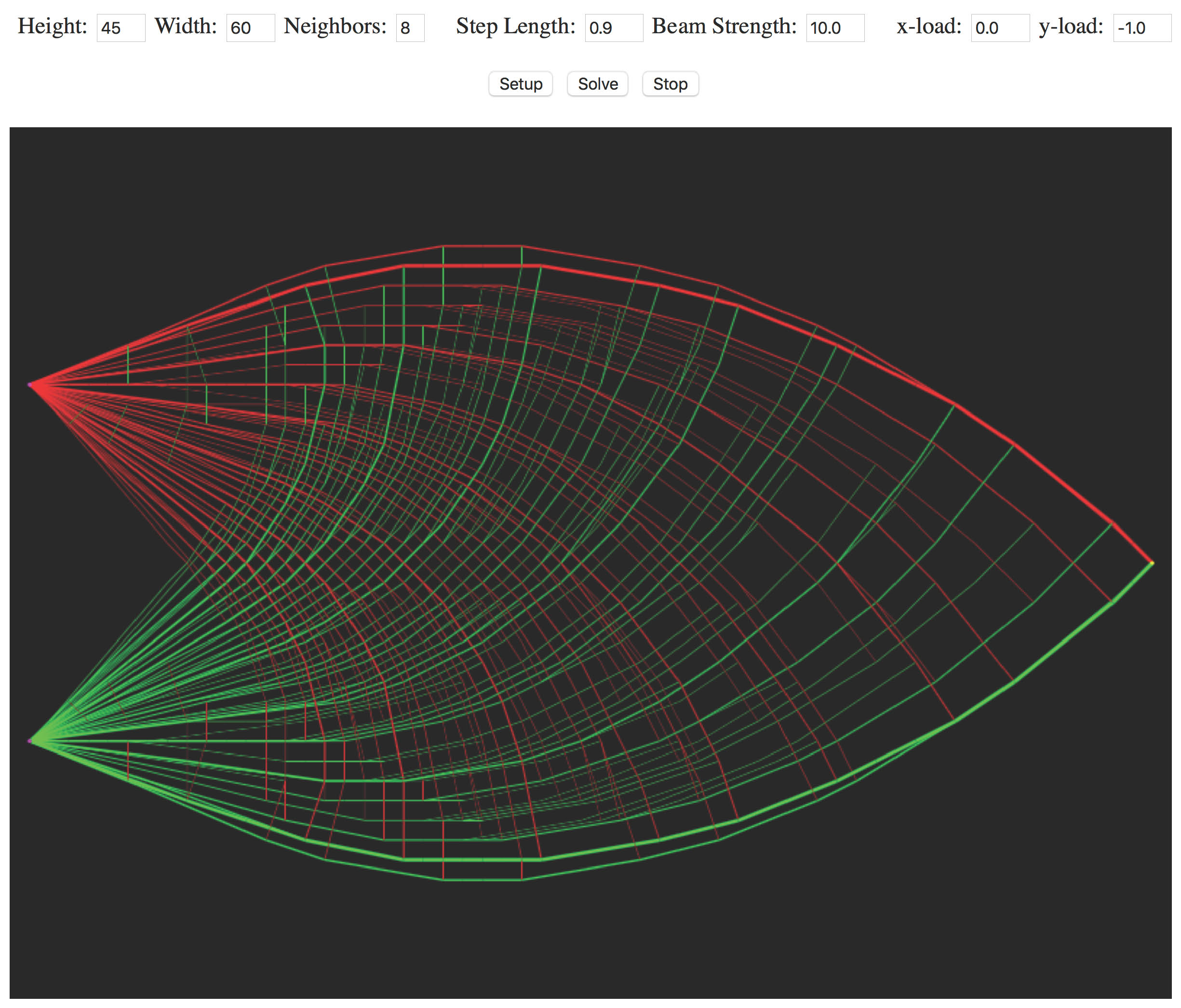
To set up a problem, first select the dimensions for the rectangular lattice
(i.e., the height and the width). Then click on the Setup button.
In setup mode, whenever you click near a node, that node gets the load
vector currently displayed in the x-load and y-load
textfields. The direction and magnitude of the load vectors are
not actually shown graphically other than
to highlight in yellow any node with a nonzero load.
Clicking near a node while holding
down the shift key tells the applet that that node is to be an anchor
node. Generally speaking, you'll need at least two anchor nodes in order
to design a stationary structure. Anchor nodes are highlighted in magenta.
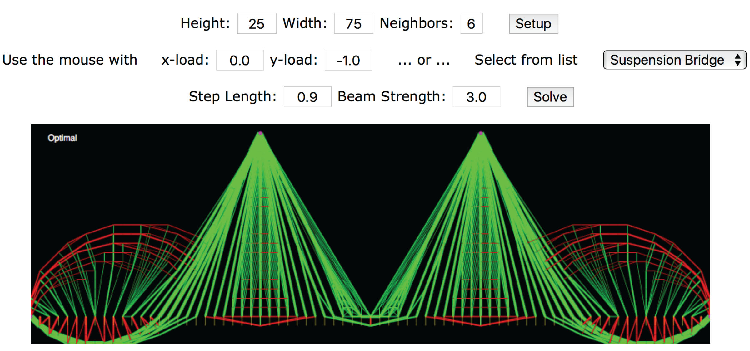
After setting the load and anchor nodes, click on solve to start the
animation.
In the optimal structure, beams with zero cross-sectional area are, of course,
simply not built. Of the beams that remain, some are under compression and
others are under tension. The compressed beams are shown in green while the
beams under tension are shown in red.
There are a few parameters that you can play with. The step length
parameter should be a number between 0 and 1. In commercial implementations
of these sorts of algorithms, the step length is taken to be very close to 1
(typically, 0.995) and the algorithm runs in very few iterations. One can
obtain a more interesting animation by setting this parameter close to
0 (say 0.1). In this case, assuming the computer you are using is fast enough,
the animation should flow like a movie going from the initial inaccurate guess
to the optimal solution.
The second parameter is the strength of the beam material.
A larger value
gives smaller cross sections. You should simply adjust this parameter as
appropriate to get a nice visual representation for each specific problem.