In a recent tech report, I derive the formula for the distribution in the complex plane of the roots of functions of the form

where the \( \alpha_j \)'s are independent standard normal (aka Gaussian) random variables and the functions \( f_j(z) \) are arbitrary analytic functions on the complex plane.

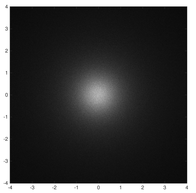
The left panel shows the theoretical expected density. The random coefficients are assumed to be iid standard Gaussian random variables. The functions \( f_j(z) \) can be selected using the pull-down menu above. The number of terms, \(n\), can also be changed.

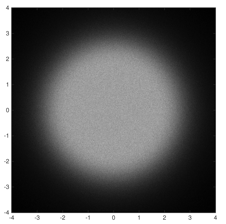
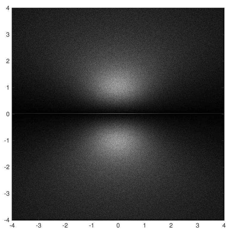
To check empirically that the theoretical distribution is correct, you can generate a large number of random polynomials and plot their roots by clicking on the Compute Empirical button. If the \(\alpha_i\)'s are standard Gaussians, then the empirical density should closely match the theoretical density (as long as the sample size is fairly large).

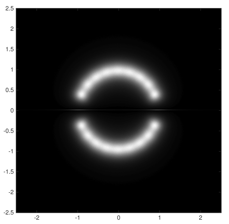
By default, 3000 random sums are generated. For large values, the empirical distribution looks very much like the theoretical density. Also, by default the functions are random polynomials. But, you can select various choices for the \( f_j \)'s including sines and cosines to make random Fourier series. You can also select a few different distributions for the \( \alpha_j \)'s but this selection only affects the empirical distribution. 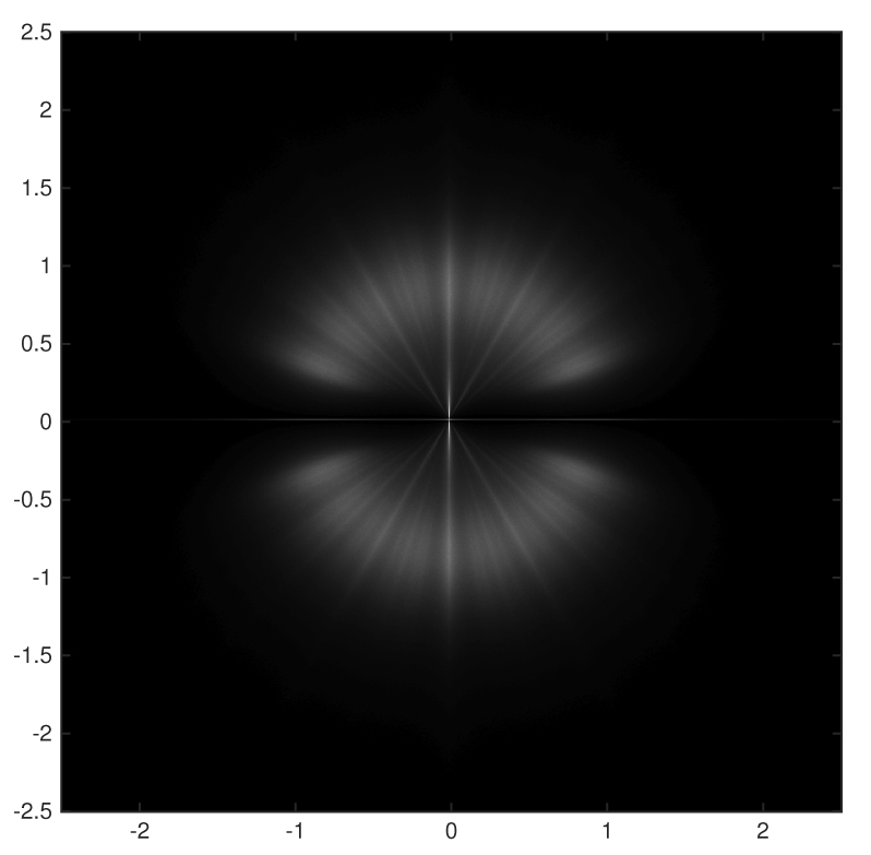The theoretical distribution always assumes a Gaussian distribution for the coefficients.

With default settings, the code takes about 15 seconds to solve (on my laptop computer). Using Matlab, one can compute the empirical distributions much more quickly. Here's the code for that: findroots.m

Here's my Java applet version (which only runs in some browsers): https://vanderbei.princeton.edu/JAVA/Roots/Roots.html

---

Here's a few screenshots of the empirical density...

Gaussian:   50 million polynomials: \( a_0 + a_1 z + \cdots + a_{10} z^{10}, \qquad a_i \in N(0,1) \)	Cauchy:   50 million polynomials: \( a_0 + a_1 z + \cdots + a_{10} z^{10}, \qquad a_i \in \mbox{Cauchy}(0,1) \)
Taylor Style:   5 million polynomials: \( a_0 + a_1 z + a_2 \frac{z^2}{2!} + \cdots + a_{10} \frac{z^{10}}{10!}, \qquad a_i \in N(0,1) \)	Uniform:   500,000 polynomials: \( a_0 + a_1 z + \cdots + a_{10} z^{10}, \qquad a_i \in \mbox{Unif}(0,1) \)
Taylor Style w/ complex coefficients:   5 million polynomials: \( a_0 + a_1 z + a_2 \frac{z^2}{2!} + \cdots + a_{10} \frac{z^{10}}{10!}, \qquad a_i \in N(0,1) + i N(0,1) \)	Root Taylor Style w/ complex coefficients:   5 million polynomials: \( a_0 + a_1 z + a_2 \frac{z^2}{\sqrt{2!}} + \cdots + a_{10} \frac{z^{10}}{\sqrt{10!}}, \qquad a_i \in N(0,1) + i N(0,1) \)

---

Updated 2016 Dec 25